📚
Summary
For Maths 1 exam click here.
For English 1 summary click here.
For Qualifier exam click here.
Week 1 to 4
Descriptive and Inferential Statistics
Descriptive Statistics: Methods for summarizing and organizing data. Examples include measures of central tendency (mean, median, mode) and measures of dispersion (range, variance, standard deviation).
Example: Calculating the mean, median, and mode of the dataset [2, 3, 3, 5, 7].
Inferential Statistics: Techniques for making predictions or inferences about a population based on a sample of data. This includes hypothesis testing and confidence intervals.
Example: Using a sample of 100 students' test scores to estimate the average test score of all students in a school.
Data Types
Categorical Data: Data that can be divided into groups or categories. Examples include gender, race, and yes/no responses.
Example: Survey responses to the question "What is your favorite color?" with options like red, blue, green, etc.
Numerical Data: Data that represents quantities and can be measured. Examples include height, weight, and age.
Example: Recording the heights of students in a class.
Scale of Measurement
Nominal: Categories without a specific order. Examples include types of fruit, colors.
Example: Classifying students by their favorite fruit: apple, banana, orange.
Ordinal: Categories with a specific order but no consistent difference between them. Examples include rankings, satisfaction levels.
Example: Ranking students as first, second, and third in a race.
Interval: Numerical data with equal intervals between values but no true zero point. Examples include temperature in Celsius or Fahrenheit.
Example: Measuring temperature in degrees Celsius.
Ratio: Numerical data with equal intervals and a true zero point. Examples include height, weight, and age.
Example: Measuring the weight of different fruits.
Frequency and Relative Frequency
Frequency: The number of times a value occurs in a dataset.
Example: Counting the number of students who scored above 90 in a test.
Relative Frequency: The proportion of times a value occurs in a dataset, calculated as frequency divided by the total number of observations.
Example: If 10 out of 50 students scored above 90, the relative frequency is 10/50 = 0.2 or 20%.
Charts
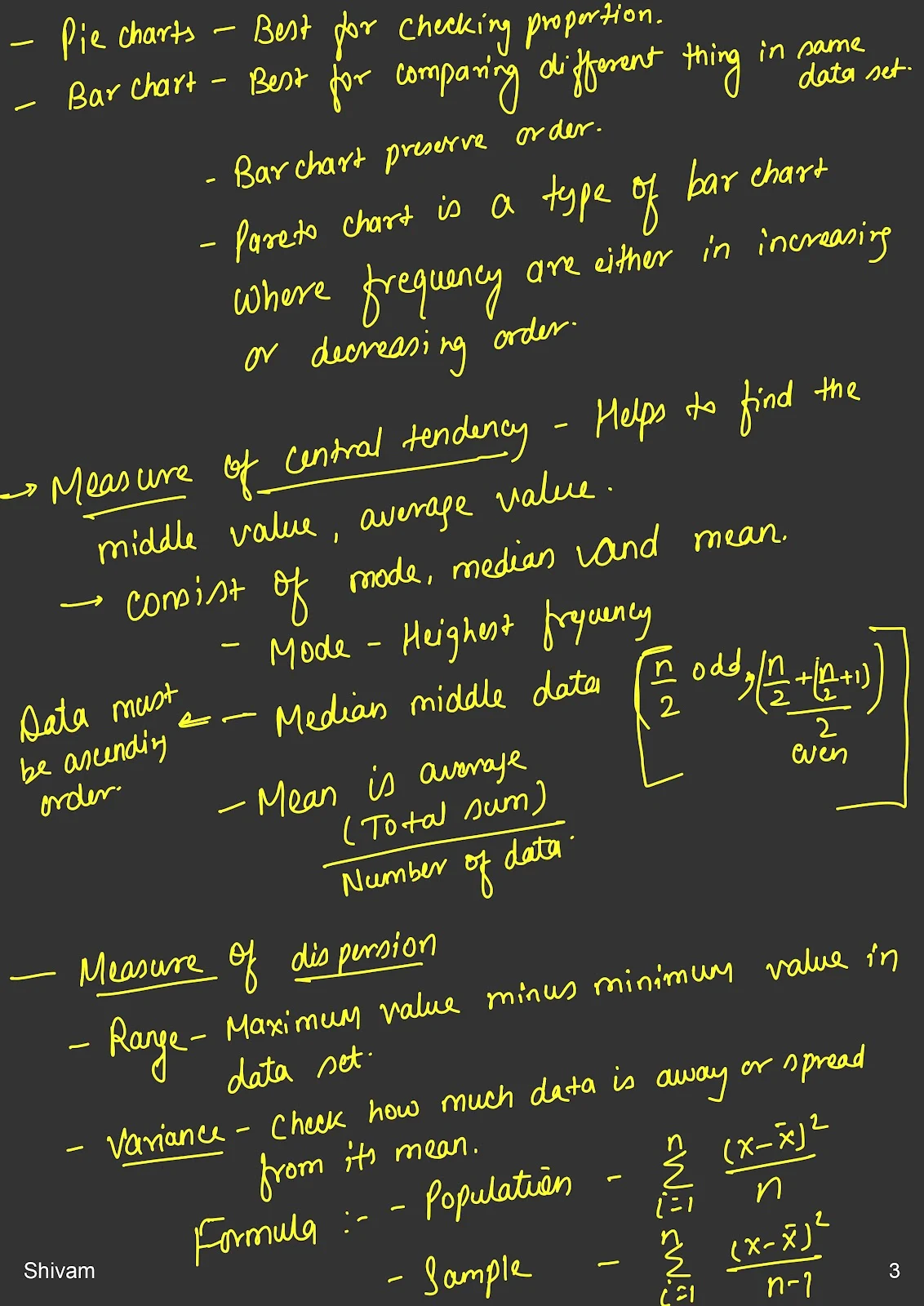
Pie Chart: A circular chart divided into sectors, each representing a proportion of the whole.
Example: A pie chart showing the distribution of favorite fruits among students.
Bar Chart: A chart with rectangular bars representing the frequency or relative frequency of different categories.
Example: A bar chart showing the number of students in different grade levels.
Pareto Chart: A bar chart where categories are ordered by frequency in descending order, often combined with a cumulative frequency line.
Example: A Pareto chart showing the most common reasons for student absences.
Measures of Central Tendency
Mean: The average of a dataset, calculated as the sum of all values divided by the number of values.
Example: The mean of the dataset [2, 3, 3, 5, 7] is (2+3+3+5+7)/5 = 4.
Median: The middle value of a dataset when the values are arranged in ascending order.
Example: The median of the dataset [2, 3, 3, 5, 7] is 3.
Mode: The most frequently occurring value in a dataset.
Example: The mode of the dataset [2, 3, 3, 5, 7] is 3.
Measures of Dispersion
Range: The difference between the highest and lowest values in a dataset.
Example: The range of the dataset [2, 3, 3, 5, 7] is 7-2 = 5.
Variance: The average of the squared differences from the mean.
Example: For the dataset [2, 3, 3, 5, 7], the variance is [(2-4)^2 + (3-4)^2 + (3-4)^2 + (5-4)^2 + (7-4)^2]/5 = 3.2.
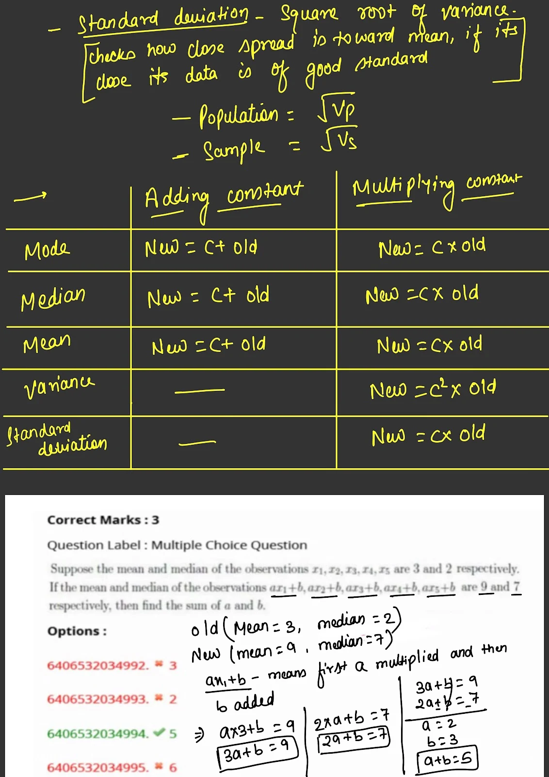
Standard Deviation: The square root of the variance, representing the average distance from the mean.
Example: The standard deviation of the dataset [2, 3, 3, 5, 7] is √3.2 ≈ 1.79.
Percentile
A measure indicating the value below which a given percentage of observations fall. For example, the 25th percentile is the value below which 25% of observations fall.
Example: In a dataset of test scores, the 90th percentile is the score below which 90% of the scores fall.
Association
Contingency Table: A table used to summarize the relationship between two categorical variables.
Example: A contingency table showing the relationship between gender (male, female) and preference for a subject (math, science).
Covariance: A measure of how two variables change together. A positive covariance indicates that the variables tend to increase together, while a negative covariance indicates that one variable tends to increase when the other decreases.
Example: Calculating the covariance between students' study hours and their test scores.
Correlation: A standardized measure of the relationship between two variables, ranging from -1 to 1. A correlation of 1 indicates a perfect positive relationship, -1 indicates a perfect negative relationship, and 0 indicates no relationship.
Example: Calculating the correlation between students' heights and weights.
Point Biserial Coefficient: A measure of the relationship between a binary variable and a continuous variable.
Example: Calculating the point biserial coefficient between gender (male, female) and test scores.
Week 5 to 8
Probability and Combinatorics
Permutation: An arrangement of objects in a specific order. The number of permutations of n objects taken r at a time is given by nPr = n! / (n-r)!
Example: The number of ways to arrange 3 out of 5 books on a shelf is 5P3 = 5! / (5-3)! = 60.
Combination: A selection of objects without regard to order. The number of combinations of n objects taken r at a time is given by nCr = n! / [r!(n-r)!]
Example: The number of ways to choose 3 out of 5 books is 5C3 = 5! / [3!(5-3)!] = 10.
Permutation vs Combination: Permutations consider order, while combinations do not.
Example: Arranging 3 books out of 5 in a specific order is a permutation problem, calculated as 5P3 = 5! / (5-3)! = 60. Choosing 3 books out of 5 without regard to order is a combination problem, calculated as 5C3 = 5! / [3!(5-3)!] = 10.
Probability
Probability: The likelihood of an event occurring, ranging from 0 (impossible) to 1 (certain).
Example: The probability of rolling a 4 on a fair six-sided die is 1/6.
Conditional Probability: The probability of an event occurring given that another event has occurred, calculated as P(A|B) = P(A and B) / P(B).
Example: The probability of drawing an ace from a deck of cards given that a king has already been drawn is 4/51.
Disjoint Events: Events that cannot occur simultaneously. The probability of either event occurring is the sum of their individual probabilities.
Example: The probability of rolling a 2 or a 5 on a fair six-sided die is 1/6 + 1/6 = 1/3.
Independent Events: Events where the occurrence of one does not affect the probability of the other. The probability of both events occurring is the product of their individual probabilities.
Example: The probability of flipping a coin and getting heads, and then rolling a die and getting a 6 is 1/2 * 1/6 = 1/12.
Total Probability: The probability of an event is the sum of the probabilities of the event occurring under different conditions, weighted by the probability of each condition.
Example: If a factory produces 70% of its products in Plant A with a defect rate of 2%, and 30% in Plant B with a defect rate of 5%, the total probability of a product being defective is (0.7 * 0.02) + (0.3 * 0.05) = 0.014 + 0.015 = 0.029 or 2.9%.
Bayes' Theorem: A formula for updating probabilities based on new information, given by P(A|B) = [P(B|A) * P(A)] / P(B).
Example: If 1% of the population has a disease and a test for the disease is 99% accurate, the probability that a person has the disease given a positive test result can be calculated using Bayes' Theorem.
Week 9 to 12
Random Variables and Distributions
Discrete Random Variable: A variable that can take on a finite or countably infinite number of values. Examples include the number of heads in coin tosses (Bernoulli, Binomial), the number of successes in a sample without replacement (Hypergeometric), and the number of events in a fixed interval (Poisson).
Example: The number of heads obtained in 10 coin tosses is a discrete random variable.
Continuous Random Variable: A variable that can take on any value within a given range. Examples include time, height, and weight.
Example: The time it takes for a student to complete an exam is a continuous random variable.
Uniform Distribution: A distribution where all outcomes are equally likely within a given range.
Example: The probability of rolling any number on a fair six-sided die is uniformly distributed.
Non-Uniform Distribution: A distribution where some outcomes are more likely than others.
Example: The probability of different grades in a class where some grades are more common than others.
Exponential Distribution: A distribution describing the time between events in a Poisson process, with a constant rate of occurrence.
Example: The time between arrivals of buses at a bus stop is exponentially distributed.
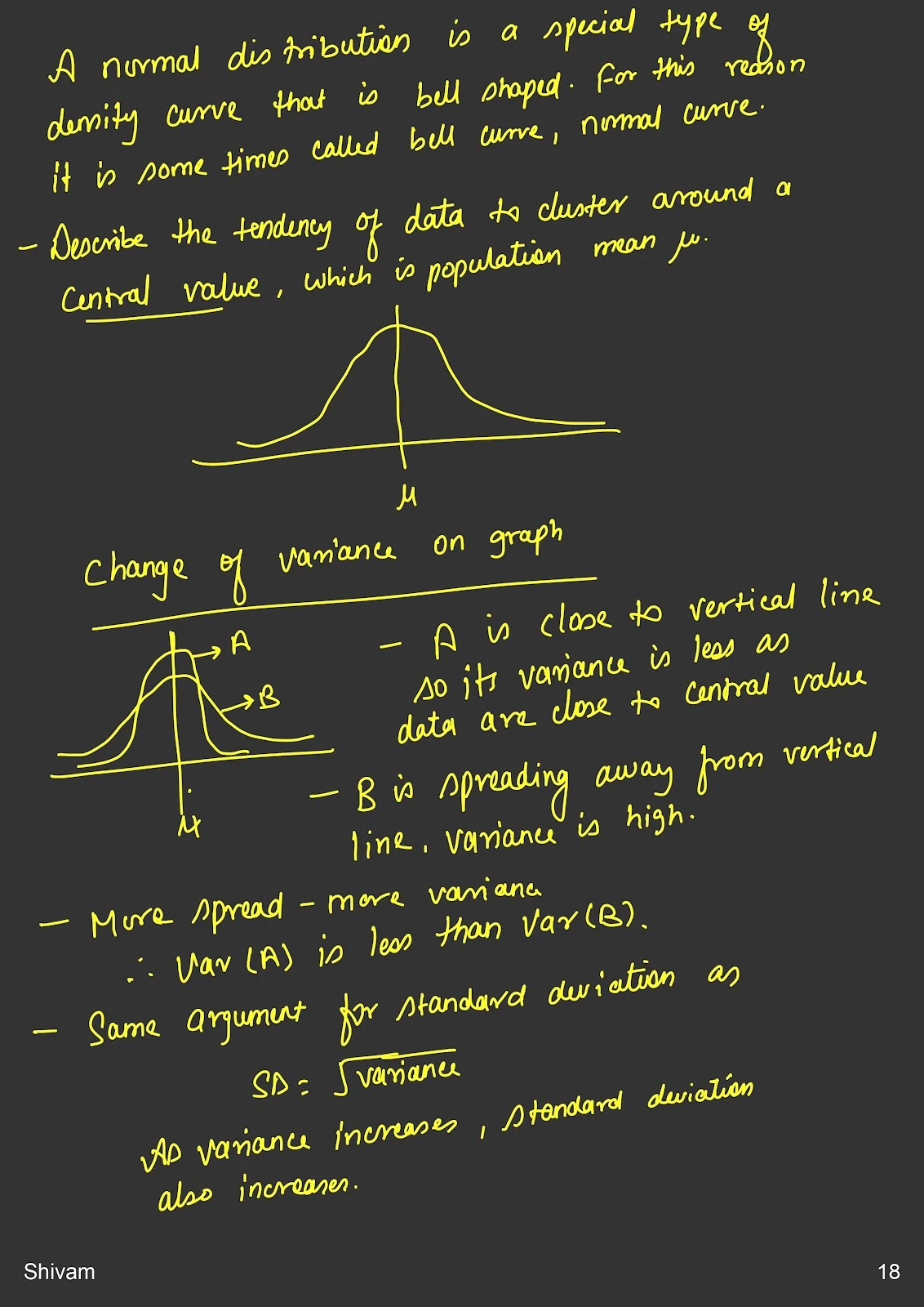
Normal Distribution: A symmetric, bell-shaped distribution characterized by its mean and standard deviation. The 68-95-99.7 rule states that approximately 68% of data falls within one standard deviation of the mean, 95% within two, and 99.7% within three.
Example: The heights of adult men in a population are normally distributed.
Standard Normal Distribution: A normal distribution with a mean of 0 and a standard deviation of 1.
Example: Standardizing a dataset of test scores to compare them to a standard normal distribution.


